
When the user draws a circle on the map and then clicks Get Draw Report, a report appears in a dialog that shows the NEPP seminars that have taken place within the area of the circle. How does this magic happen?

The first thing to understand is that there are two softwares combining with each other here, Google Maps and the PostGIS extension of the PostgreSQL database, and that they don’t automatically know about each other. This is different than the Microsoft environment where softwares are connected to each other and thus “know” about each other. This may seem like a good thing, but in reality it causes complexity that often causes problems with the softwares.
For example, recently at the my place of work an install of SQL Server 2008 Management Studio caused Visual Studio 2008 to fail. We then installed Managment Studio on a virtual machine where there was no other Microsoft software, and the software worked as it should. Having softwares “know” about each other violates the OO principles of “loose coupling” and “tight cohesion”. Software functions best when it is independent of other software.
In this case, Google Maps must expose enough information about its circle so that PostGIS can recreate the circle and query the database for those seminars that fall within the circle. Google Maps exposes two facts about its circle, the radius of the circle and the center point. Having those two facts, the browser uses the Google geometry library to also find the four points to the north, south, east, and west of the radius of the circle:
spherical = google.maps.geometry.spherical;
center = selectedShape.getCenter();
radius = selectedShape.getRadius();
north = spherical.computeOffset(center, radius, 0);
east = spherical.computeOffset(center, radius, 90);
south = spherical.computeOffset(center, radius, 180);
west = spherical.computeOffset(center,radius,270);
The browser now performs an AJAX query and sends these four points to the server side PHP program. PHP uses these four points to construct a spatial query to the database. The WHERE clause of the query illustrates the complex spatial operations of which PostGIS is capable:
WHERE
ST_WITHIN
(
  geometry,
  ST_MAKEPOLYGON
  (
    ST_CURVETOLINE
    (
      ST_GEOMFROMTEXT
      (
       'SRID=4326;
        CIRCULARSTRING
        (
           -123.1199 49.2662,
           -123.1098 49.2727,
           -123.0998 49.2662,
           -123.1098 49.2596,
           -123.1199 49.2662
        ) – end CIRCULARSTRING
      ') -- end ST_GEOMFROMTEXT
    ) -- end ST_CURVETOLINE
  ) -- end ST_MAKEPOLYGON
) -- end ST_WITHIN
This query first creates a CIRCULARSTRING, which is a curved string that begins and ends on the same point. The CIRCULARSTRING acts as input to ST_GEOMFROMTEXT, which makes a valid geometry object, using the spatial reference id (SRID) for WGS84, which is what Google Maps uses.
The geometry object then acts as input to ST_CURVETOLINE. This function converts a CIRCULARSTRING to a valid polygon, with a default value of 128 segments. This is because PostGIS does not actually do a spatial query with a circle, but rather with an approximation of a circle.
Finally the polygon acts as input to ST_WITHIN, which PostGIS uses to retrieve features within the polygon.
PHP retrieves the results of the spatial query, formats it as an HTML table and sends it back to the browser. The browser invokes a jQuery dialog and outputs the HTML table to the dialog.
In conclusion a Google circle is not the same as a PostGIS circle. These two softwares are independent of each other, but must be able to communicate in a non-partisan way to all other softwares. This they do extremely well.
 First, look at the Renters layer. This layer shows us that many people in the West End (the red part in top left), a densely packed area of 100,000 people in 100 square blocks, rent their dwelling units.
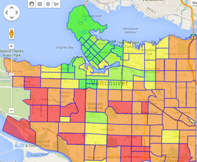
 Finally, look at the Family – average size layer. This layer is similar to the Population – 14 years and under layer; the south part of Vancouver has large families, while in the West End, families are not large.